Dynamic Programming 
| Prerequisites: | Preliminaries | Hello-world |
In this exercise you will implement Value and Policy iterations to solve Markov Decision Processes (MDPs). The exercise has two parts. In Part 1 you model a grid-world problem as an MDP and solve it. In Part 2 the world changes in three small ways, and each change quietly breaks the Markov property of the grid: knowing the robot’s cell is no longer enough to predict its future. Your job, for each case, is to figure out what the state needs to remember, turn the problem back into an MDP, and solve it with the very same Value and Policy Iteration you wrote for Part 1.
You are an operator on a distant planet at a base responsible for deploying autonomous survey robots looking for unobtainium. Your job is to send a surveying robot to a location specified by your company’s client.
For each contract, you can deploy several robots, but only one at a time - corporate requires you to have at most one active robot in the field at any given time to try to save money. You can always choose to abandon an active robot and deploy a new one from the base. In some cases, an active robot might break down - then, you are forced to abandon it. However, deploying the second and every next robot for a contract costs you money (the first robot is covered by the client).
Once a robot reaches the goal location, it stays there and delivers data reports to the client, thus fulfilling the contract. For this, you receive a reward from the client. Your robot should reach the goal location as fast as possible since the client is entitled to compensation for the time it takes you to fulfill the contract.
Your task is to create a plan for each given contract that maximizes your profit. You choose to model this problem as a Markov Decision Process (MDP) and use dynamic programming to compute offline the optimal policy for each mission.
Part 1: the base problem
The world is modeled as a 2D grid, which is represented through a MxN matrix (numpy array). Rows and columns represent the $i$ and $j$ coordinates of the robot, respectively. The area around you is a tropical rainforest, which can be modeled in the grid with the following types of cells:
-
GRASS(green) - it will take the robot 1 hour to cross this cell. -
SWAMP(light blue) - it will take the robot 2 hours to cross this cell. -
CLIFF(black) - untraversable cell. If the robot tries to move in this cell, it will break down and you will need to deploy a new robot from the base. -
GOAL(red) - the goal location you need to survey. -
START(yellow) - the location of your base, it can be considered aGRASScell. The 8 cells close to theSTARTcell are alwaysGRASSorGOALcells, except for the 4 in the corners that could also beSWAMP, and there are at least 2 cells between theSTARTcell and the edge of the map or aCLIFFcell. In other words, the robot will never break down in theSTARTcell and the four neighboring cells.
The time required to cross each cell corresponds to the time a robot needs to leave this cell
(e.g. leaving the START cell takes 1 hour).
When in a specific cell, you can plan for the robot to take one of the following actions:
- move in a selected direction:
SOUTH, NORTH, EAST, WEST - give up and
ABANDONits mission (this implies the deployment of a new robot from the base), -
STAYif arrived at theGOAL.
The goal of your policy is to maximize profit (use 1k USD as the default unit):
- You keep receiving a bonus of 50k USD for your robot surveying (staying at) the goal location.
- For each hour of the time it takes you to fulfill the contract, your client is entitled to a compensation of 1k USD. No compensation is paid if the robot is already at the goal location.
- The deployment of each new robot costs you 10k USD (the first robot is covered by the client).
The planet’s atmosphere is very foggy and when the robot decides to move in a specific direction, it may not end up where initially planned. Sometimes, when trying to move, it might also break down and be forced to abandon its mission. In fact, for all transitions, the following probabilities are given:
- In
GRASS:- If the robot chooses to move (
SOUTH, NORTH, EAST, WEST), the chosen transition will happen with a probability of 0.75. The remaining 0.25 is split among the other 3 movement transitions. The robot will not break down in this cell. - If the robot chooses to give up, it will
ABANDONits mission with probability 1.0.
- If the robot chooses to move (
- In
SWAMP:- Because it is harder to move, if the robot chooses to move
(
SOUTH, NORTH, EAST, WEST), the chosen transition will happen with a probability of 0.5. With probability 0.25, the robot will move to one of the other neighboring cells (with all of them equally likely). With probability 0.2, the robot will not be able to move out of the cell (it will stay in the cell). With probability 0.05 the robot will break down and will need toABANDONits mission. - If the robot chooses to give up, it will
ABANDONits mission with probability 1.0.
- Because it is harder to move, if the robot chooses to move
(
- In
CLIFF:- The robot will break down with probability 1.0.
- When in the
GOALthe robot willSTAYwith probability of 1.0. - The robot cannot directly pick an action that would take it outside the map or to a
CLIFFcell. However, it may be that the robot ends up out of the map or in aCLIFFcell as described by the movement transition probabilities above. If this happens, the robot breaks down.
If the robot breaks down or chooses to ABANDON the mission, a new robot is deployed in
the START cell, which costs you 10k USD.
Hints
- You can model the
ABANDONaction transition as a transition in your MDP from the current cell to theSTARTcell with the cost of deploying a new robot. - If the robot chooses a movement action in any cell, it will take it the time specified for
this cell type to try to perform this action. An attempt to move out of the
SWAMPcell always takes 2 hours, even if the robot ends up staying in the cell or breaking down. - Note that the robot will never break down in the
STARTcell or in its four neighboring cells because of the assumptions on their type and location on the map.
Part 2: new states
Everything above still holds. In each of the three cases below, one short story change breaks
the Markov property of the bare grid; you decide what the state must remember to restore it.
The state becomes (i, j, z) where z is defined per case, and your value function and
policy become arrays of shape (M, N, Z): one grid slice per value of z. Each case is
solved and graded separately.
Case 1: Forecast (“the base radios the fog”)
Each hour the base transmits a forecast for the coming hour’s fog. Forecasts are independent
across hours, with P(FOGGY) = 0.3. The forecast does not change the world; it only tells
you how this hour’s move will behave:
| forecast f | GRASS intended / each slip | SWAMP intended / each slip | stay | break |
|---|---|---|---|---|
| CLEAR | 0.75 / 0.25 ÷ 3 (as in Part 1) | 0.50 / 0.25 ÷ 3 | 0.20 | 0.05 |
| FOGGY | 0.55 / 0.15 | 0.30 / 0.15 | 0.20 | 0.05 |
(The forecast’s accuracy is already folded into these numbers.) Think carefully about whether something that changes nothing physical still needs to be part of the state.
Case 2: Momentum (“the robot keeps rolling”)
The robots’ wheels carry momentum: slips lean toward wherever the robot moved last hour, and turning around against your own motion is hard.
Let h be the direction the robot actually moved last hour, one of
{-, NORTH, WEST, SOUTH, EAST}, where - means it did not move (it stayed in place, or a
fresh robot was just deployed). When the robot chooses a movement action u:
The movement outcomes are: the intended direction u, a slip toward h (when it
differs from u), and a slip to each remaining direction. Depending on how h relates
to u:
-
h = -: no momentum; exactly the Part-1 distribution. -
h = u: intended +0.10; the remaining movement mass splits uniformly, 0.05 per other direction. -
hopposite ofu: intended -0.10; the slip leans backward: 0.25 towardh, 0.05 toward each perpendicular direction. -
hperpendicular tou: intended unchanged; the slip leans sideways: 0.15 towardh, 0.05 toward each of the other two directions.
For example, on GRASS this gives:
| last heading h | intended u | slip toward h | each remaining direction |
|---|---|---|---|
- (no momentum) |
0.75 | - | 0.25/3 each (3 directions) |
| h = u (same direction) | 0.85 | - | 0.05 each (3 directions) |
| h opposite of u | 0.65 | 0.25 | 0.05 each (2 directions) |
| h perpendicular to u | 0.75 | 0.15 | 0.05 each (2 directions) |
As in Part 1, a slip that would take the robot off the map or into a CLIFF cell is a
breakdown (a new robot is deployed at START).
After the hour: h becomes the direction the robot actually moved - not the one you
commanded. If you command EAST and the robot slips NORTH, next hour h = NORTH. If it
stayed in place, or broke down, or you chose ABANDON (a fresh robot is deployed at START,
and a fresh robot has no momentum), then h = -.
Case 3: Glitch (“bad wheel days”)
The robots’ wheels sometimes glitch, and once the glitching starts it tends to last a while.
Let g in {OK, GLITCHY} be the current condition of the wheels.
How the robot moves this hour depends on the current g:
-
g = OK: exactly the Part-1 distribution. -
g = GLITCHY: the intended probability drops by 0.15 and the freed mass splits uniformly over the other 3 directions (0.05 more per slip). OnGRASS: 0.60 intended, 0.40/3 per slip. OnSWAMP: 0.35 intended, 0.40/3 per slip; stay (0.20) and break (0.05) are unchanged.
Unlike the forecast, the glitch has memory. At the end of the hour g evolves:
- after a normal hour (the robot moved or stayed in place):
P(OK -> GLITCHY) = 0.1andP(GLITCHY -> OK) = 0.3; - after a breakdown or
ABANDON, a fresh robot is deployed atSTART, and a fresh robot has new wheels:g = OKwith probability 1, whatever the old robot’s wheels were doing.
Something to think about. Before writing code for each case, try to answer for yourself: what is your state, why does the grid alone stop being Markov, and why does your state restore it? A wrong state choice is much easier to catch in a few sentences than in a heatmap.
Tasks
Data structure
Actions, states, Value function and Policy are defined as follows (exercises/ex04/structures.py):
@unique
class Action(IntEnum):
    NORTH = 0
    WEST = 1
    SOUTH = 2
    EAST = 3
    STAY = 4
    ABANDON = 5


State = tuple[int, int]
"""The Part-1 state is a tuple of two ints."""


@unique
class Cell(IntEnum):
    GOAL = 0
    START = 1
    GRASS = 2
    SWAMP = 3
    CLIFF = 4


AugmentedState = tuple[int, int, int]
"""The Part-2 state is (i, j, z); z orderings are fixed by these enums:"""


@unique
class Heading(IntEnum):
    NONE = 0; NORTH = 1; WEST = 2; SOUTH = 3; EAST = 4

@unique
class Fog(IntEnum):
    CLEAR = 0; FOGGY = 1

@unique
class Gear(IntEnum):
    OK = 0; GLITCHY = 1


ValueFunc = NDArray[np.float64]   # (M, N) in Part 1, (M, N, Z) in Part 2
Policy = NDArray[np.int64]        # (M, N) in Part 1, (M, N, Z) in Part 2

OptimalActions = NDArray[np.object_]
"""
Type Alias for the all optimal actions per state. It is a numpy array of list objects where
each list contains the optimal actions that are equally good for a given state. It is the
type of the ground truth policy that your solution will be compared against. You are not
required to use this type in your solution.
"""
The MDP models
The first subtask is to implement the missing methods in exercises/ex04/mdp.py.
These methods will be useful when implementing value and policy iteration.
For each class you need to fill in get_transition_prob, which returns the probability of
transitioning from a state to another given an action, and stage_reward, which returns the
reward for that transition. The signatures are identical across all four classes; only the
State widens to AugmentedState in Part 2:
class GridMdp:
    def __init__(self, grid: NDArray[np.int64], gamma: float = 0.9):
        assert len(grid.shape) == 2, "Map is invalid"
        self.grid = grid
        """The map"""
        self.gamma: float = gamma
        """Discount factor"""

    def get_transition_prob(self, state: State, action: Action, next_state: State) -> float:
        """Returns P(next_state | state, action)"""
        # todo

    def stage_reward(self, state: State, action: Action, next_state: State) -> float:
        # todo


class MomentumGridMdp(AugmentedGridMdp): ...   # Z = 5
class FogGridMdp(AugmentedGridMdp): ...        # Z = 2
class GlitchGridMdp(AugmentedGridMdp): ...     # Z = 2
Feel free to add more methods in case you need to.
You must not change the names and signatures of get_transition_prob and stage_reward.
Value Iteration
We’ll start with value iteration. You need to implement the solve method in
exercises/ex04/value_iteration.py:
class ValueIteration(GridMdpSolver):
    @staticmethod
    @time_function
    def solve(grid_mdp: AnyGridMdp) -> tuple[ValueFunc, Policy]:
        value_func = np.zeros_like(grid_mdp.grid).astype(float)
        policy = np.zeros_like(grid_mdp.grid).astype(int)

        # todo implement here

        return value_func, policy
Policy iteration
For policy iteration, you need to implement the solve method in
exercises/ex04/policy_iteration.py:
class PolicyIteration(GridMdpSolver):
    @staticmethod
    @time_function
    def solve(grid_mdp: AnyGridMdp) -> tuple[ValueFunc, Policy]:
        value_func = np.zeros_like(grid_mdp.grid).astype(float)
        policy = np.zeros_like(grid_mdp.grid).astype(int)

        # todo implement here

        return value_func, policy
(For Part 2 you will need arrays of shape (M, N, Z) instead - adapt the initialization
accordingly.)
One solver serves both parts: if you write it to iterate over “the states of the MDP” it runs on Part 2 unchanged; only the model underneath grows.
Expected outcome
For both Value and Policy iterations, you need to return the optimal ValueFunc and
one of the optimal Policy for the given MDP.
Note: The optimal value function is unique, but the optimal policy is not. You can return any optimal policy that satisfies the Bellman optimality equation; the ground truth stores all optimal actions per state, so your tie-breaking never costs you.
To keep the format consistent, the value function and policy should be returned as numpy
arrays where each cell corresponds to the value of the state or the action to be taken in the
state, respectively: MxN matrices in Part 1 and MxNxZ arrays in Part 2. The value
function and policy of CLIFF cells will be excluded for evaluation. This is because you are
never in CLIFF.
If your algorithm works, in the report you should find some results similar to this:
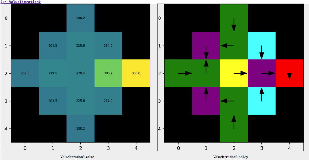
Figure 1: Visualization of the optimal value function and policy for the 5x5 example.
On the left the Value function is visualized as a heatmap.
On the right you can see the map with the original cells and the corresponding optimal policy
(arrows for movement actions, X for the ABANDON action, a dot for STAY at the goal).
Help for modeling the MDP
Correctly modeling the MDPs is crucial. For Part 1 we provide the admissible action set and
ground truth transition probabilities and rewards for selected cells of the
5x5 example map;
for Part 2, get_transition_prob is additionally evaluated on sampled augmented triples.
The coordinates of the cells are given in the format (row, column) starting from the top
left corner of the grid. All axes are 0-indexed.
Admissible action set (Part 1, 5x5 example)
<current state>: [list of admissible actions]
- (0, 1): [SOUTH, EAST, ABANDON]
- (1, 2): [NORTH, WEST, SOUTH, EAST, ABANDON]
- (2, 0): [NORTH, SOUTH, EAST, ABANDON]
- (4, 3): [NORTH, WEST, ABANDON]
Ground truth transition probabilities and rewards (Part 1, 5x5 example)
(<current state>, <action>): (<next state>, <probability>, <reward>)
- ((0, 1), SOUTH):   ((1, 1), 0.75, -1), ((0, 2), 0.0833, -1), ((2, 2), 0.1667, -11)
- ((0, 1), ABANDON): ((2, 2), 1.0, -10)
- ((1, 2), WEST):    ((1, 1), 0.75, -1), ((0, 2), 0.0833, -1), ((1, 3), 0.0833, -1), ((2, 2), 0.0833, -1)
- ((2, 0), SOUTH):   ((3, 0), 0.75, -1), ((1, 0), 0.0833, -1), ((2, 1), 0.0833, -1), ((2, 2), 0.0833, -11)
- ((3, 3), WEST):    ((3, 2), 0.5, -2), ((2, 3), 0.0833, -2), ((3, 4), 0.0833, -2), ((4, 3), 0.0833, -2), ((3, 3), 0.2, -2), ((2, 2), 0.05, -12)
Test cases and performance criteria
The algorithms are going to be tested on different MDPs of both parts. The public test set contains three maps: the 5x5 example plus randomly generated 10x10 and 40x40 maps.
If you want broader coverage, set ALL_MAPS = True at the top of
exercises_def/ex04/ex04.py to run the same tests and metrics on three additional smaller
maps (6x6, 9x9 and 12x12, with published solutions) on top of the three public ones.
For even more maps to experiment on, random_map(shape, seed=...) in
exercises_def/ex04/map.py generates random maps with the goal guaranteed reachable.
You will be able to test your algorithms on some test cases with given solution, the outputted Policy and ValueFunc will be compared to the solution.
After running the exercise, you will find the reports in out/04/ for each test case.
There you will be able to visualize the MDPs, your output and the expected solution; Part-2
reports show one heatmap per z slice, so you can see how the optimal route changes between a
CLEAR and a FOGGY forecast, or how momentum makes the robot prefer not to turn around.
These test cases are not graded but serve as a guideline for how the exercise will be graded overall.
The final evaluation will combine the following metrics: ratio of completed cases, transition_prob_accuracy, average policy_accuracy, average value_func_R2, and average solve_time:
- ratio of completed cases: $\frac{N_{completed}}{N}$
- transition_prob_accuracy: This metric will evaluate the accuracy of your transition probability, in particular, for different cases (state, action, next_state), it considers 1.0 if the probability is equal (up to numerical errors) to the ground truth, 0.0 otherwise. Then it averages the results.
-
policy_accuracy: This metric will evaluate the accuracy of your
Policy, in particular, it averages for each state of the MDP the number of correct actions (# of correct actions)/(# of states). An action counts as correct if it is any optimal action of that state, so your tie-breaking never costs you. Thus, policy_accuracy will be in the interval [0, 1]. -
value_func_R2: This metric will evaluate the accuracy of your
ValueFunc. It is a measure of how well yourValueFuncapproximates the ground truthValueFunc. It is computed as $R^2 = 1 - \frac{\sum_{s \in S} (VF^{gt}(s) - VF(s))^2}{\sum_{s \in S} (VF^{gt}(s) - \bar{VF^{gt}})^2}$ where $VF^{gt}$ is the ground truthValueFunc, $VF$ is yourValueFunc, and $\bar{VF^{gt}}$ is the mean of the ground truthValueFunc. With negative values being clipped to 0, this metric will be in the interval [0, 1]. - solve_time: As your algorithms will be tested on MDPs of increasing size, the efficiency of your code will be measured in terms of process time required (in seconds).
The value function and policy of CLIFF cells are excluded from the evaluation.
Note: both algorithms must be your own implementations.
For reference, the TA’s solution achieves the following on the server, averaged over all Part-1 and Part-2 test cases (its policy_accuracy, value_func_R2 and transition_prob_accuracy are all 1.0):
| Algorithm | Solve time [s] |
|---|---|
| ValueIteration | 0.500 |
| PolicyIteration | 0.423 |
Use these numbers as a guideline for the order of magnitude of a correct, plainly written implementation (Python loops over dictionaries, no vectorisation).