Informed Graph Search 
| Prerequisites: | Preliminaries | Hello-world |
|---|
Informed graph search
In this exercise we look at weighted graph and related search algorithms for finding the shortest path. Specifically, you are tasked with the implementation of two algorithms: Uniform Cost Search (UCS) and A*.
Graph structures
In this exercise we need to augment the AdjacencyList seen in Exercise
2
to keep track of the weights on the edges. A simple extension is the following:
@dataclass
class WeightedGraph:
    adj_list: AdjacencyList
    weights: Mapping[Tuple[X, X], float]
    _G: MultiDiGraph

    def get_weight(self, u: X, v: X) -> Optional[float]:
        """
        :param u: The "from" of the edge
        :param v: The "to" of the edge
        :return: The weight associated to the edge, raises an Exception if the edge does not exist
        """
        try:
            return self.weights[(u, v)]
        except KeyError:
            raise EdgeNotFound(f"Cannot find weight for edge: {(u, v)}")

    def _get_node_attribute(self, node_id: X, attribute: NodeAttribute) -> Any:
        """
        Private method of class WeightedGraph
        :param node_id: The node id
        :param attribute: The node attribute name
        :return: The corresponding value
        """
        return self._G.nodes[node_id][attribute]

    def get_node_coordinates(self, u: X) -> Tuple[float, float]:
        """
        Method of class WeightedGraph:
        :param u: node id
        :return (x, y): coordinates (LON & LAT) of node u
        """
        return self._G.nodes[u][NodeAttribute.LONGITUDE], self._G.nodes[u][NodeAttribute.LATITUDE]
We will be using connectivity graphs of a few (famous) cities around the world; sometimes, these cities will also be connected to their nearest neighboring cities (you can find a clue on how this is done in the file ‘exercises_def/ex03/data.py’).
In order to properly implement your algorithms, you will need to get some property from the nodes (e.g., their position on the map).
You can access a nodes coordinate using the method get_node_coordinates().
The edge weight between 2 nodes is given as the travel time required to go from a node to the other, and it is directly retrievable with the function get_weight().
Task
Implement the following algorithms in src/pdm4ar/exercises/ex03/algo.py:
@dataclass
class UniformCostSearch(InformedGraphSearch):
    def path(self, start: X, goal: X) -> Path:
        # todo
        pass

@dataclass
class Astar(InformedGraphSearch):

    # ...provided code...

    def _INTERNAL_heuristic(self, u: X, v: X) -> float:
        # todo
        return 0

    def path(self, start: X, goal: X) -> Path:
        # todo
        return []
Unlike UCS, A* is an informed algorithm thus requires implementing a heuristic function. While worst time complexity is the same for UCS and A*, the use of an admissible heuristic often leads to a lower number of explored nodes to find the shortest path. If not path is found, your algorithms should return an empty list.
You are free to implement the _INTERNAL_heuristic function based on any metric of your choice (make sure it is admissible!).
There exist many distance metrics. Below is provided a visual representation of the most common.
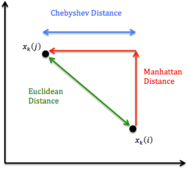 image reference
As mentioned, the edge weight between 2 nodes is given as travel time. There’s a finite number (4) of speed regimes that can be followed along an edge, as represented in the class below.
You can access the speed value using the .value property of the struct, i.e. HIGHWAY.value.
@unique
class TravelSpeed(float, Enum):
    HIGHWAY = 100.0 / 3.6
    SECONDARY = 70.0 / 3.6
    CITY = 50.0 / 3.6
    PEDESTRIAN = 5.0 / 3.6
You are NOT allowed to use any existing graph search function implemented in the libraries such as networkx.
In addition to evaluating the correctness of your path, we will also evaluate your heuristic. If you choose a good heuristic, your algorithm will explore fewer nodes, and therefore your heuristic will be called less often. Therefore, the number of times your heuristic is called provides a good metric for your algorithm’s efficiency. We will plug your heuristic function into our Astar solution and count how many times it is called. As a baseline, we will compare it with the “trivial” heuristic, which always returns 0 (this is algorithm is equivalent to UCS). We refer to the ratio of these values as the “heuristic efficiency”. With a well chosen heuristic, your efficiency should be below 1.
To get a sense of your heuristic efficiency, you can judge its performance on your own implementation of Astar. Every time you want to calculate the heuristic in path, make sure you call the heuristic function. Then, the evaluator will then run your Astar algorithm in two different modes. In the first run, the heuristic function will call the function that you implemented in _INTERNAL_heuristic. In the second mode, heuristic will simply return 0. The number of calls to the heuristic in each mode is printed in the tester output. Note that the heuristic efficiency calculation depends on the specific implementation of Astar. Therefore your local values might differ from the server’s results. Nevertheless, this should tell you if you’re on the right track.
(HINT 1) The edge weight is the travel time between the 2 nodes, hence you should think about converting travel distance into travel time. Under which condition will the time metric be admissible?
(HINT 2) To obtain the distance between 2 coordinates, you may find useful the function osmnx.distance.great_circle_vec().
(HINT 3) For UCS and Astar, you may find Python’s heapq module useful.
(HINT 4) You might want to organise your queue as queue = [ (<priority>, <i = insertion order>, <node>, <cost-to-reach>, <parent_node>) ]
In addition, we provide you with a script to allow you to increase and personalise your local test cases on the existing graphs. You can choose the (start_node, goal_node) tuples of int as query for your search algorithm without worrying they actually exist, as they will be checked and filtered. Moreover, a predefined function will generate existing random queries if you set a positive integer in the n_random_queries dict. Edit src/pdm4ar/exercises_def/ex03/local_queries.py in the apposite window:
def get_local_queries(G: WeightedGraph, id: str) -> set[Query]:
    """
    Generate local queries for the given graph.
    Local queries are manually specified node pairs.
    Random queries are sampled from adjacent node pairs in the graph.
    """

    # === STUDENT-EDITABLE SECTION ===

    my_queries = {"ny": set(),
                  "eth": set(),
                  "milan": set()}                           # Replace set() with e.g.{(1, 2), (3, 4)}
    n_random_queries = {"ny": 0, "eth": 0, "milan": 0}      # Replace 0 with another int
    random_seed = None                                      # Set an integer if you want deterministic results

    # === END STUDENT-EDITABLE SECTION ===
Test cases and performance criteria
The algorithms are going to be tested on different graphs, each containing randomly generated queries (start & goal node).
You will be able to test your algorithms on some test cases with given solution, the outputted Path will be compared to the solution.
After running the exercise, you’ll find reports in out/[exercise]/ for each test case. There you’ll be able to visualize the graphs, your output and the solution.
These test cases are not graded but serve as a guideline for how the exercise will be graded overall.
The final evaluation will combine 3 metrics lexicographically <number of solved cases, accuracy, efficiency>:
-
Accuracy: Both UCS and A* will be evaluated. A
Pathto be considered correct has to fully match the correct solution. Averaging over the test cases we compute an accuracy metric as (# of correct paths)/(# of paths). Thus, accuracy will be in the interval [0, 1]. - Efficiency: Your efficiency score will incorporate both the solve time and the heuristic efficiency. A simple heuristic should suffice. After all, choosing a computationally complex heuristic might affect the solve time.
For reference, the TA’s solution achieves the following efficiency and solving times on the server:
| Metric | Values |
|---|---|
| Heuristic efficiency | 0.6112 |
| Solve time [s] | 0.0102 |
Use these numbers as a guideline to understand the order of magnitude of expected performance for a decently optimized solution.
Useful remarks from last year Q&A
- Please, use the provided templates to implement your functions, without modifying the arguments and output numbers and types, unless stated otherwise.
- If not explicitly instructed otherwise, you may use anything included in the Docker environment to simplify your calculations.
- Since Uniform Cost Search is a special case of the A* algorithm, it is allowed to use A* implementation for UCS too, writing the code in the correct place and setting heuristic function = 0.
- BE CAREFUL: in the A* algorithm, the heuristic is summed to the cost-to-reach only for the ranking step in the queue, but you must not update the cost-to-reach with the heuristic estimate!
- For debugging, please keep in mind that your code has to work in all possible scenarios. Find them all!